quaternions versus elementary matrices

The best way to get this point of view, and at the same time give the whole topic of $2x2$ matrices an elegent formulation, is to use quaternions. Starting from the natural basis for $2x2$ matrices,

$$\begin{eqnarray*} {\bf e}_{11} & = & \left[ \begin{array}{cc} 1 & 0 \\ 0 & 0 \en... ... & \left[ \begin{array}{cc} 0 & 0 \\ 0 & 1 \end{array} \right]. \end{eqnarray*}$$

whose rule of multiplication is 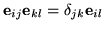${\bf e}_{ij} {\bf e}_{kl} = \delta_{jk} {\bf e}_{il}$, quaternion-like matrices can be defined by

$$\begin{eqnarray*} {\bf 1}& = & \left[ \begin{array}{cc} 1 & 0 \\ 0 & 1 \end{arr... ...& \left[ \begin{array}{cc} 1 & 0 \\ 0 & -1 \end{array} \right]. \end{eqnarray*}$$

In detail,

$${\bf 1}= {\bf e}_{11} + {\bf e}_{22}, {\bf i}= {\bf e}_{12} -... ...f e}_{12} + {\bf e}_{21}, {\bf k}= {\bf e}_{11} - {\bf e}_{22},$$

all built from sums and differences, thereby retaining real matrices. Like quaternions, these matrices anticommute (except for the identity), so the difference is that only one square is $-{\bf 1}$, the others are $+{\bf 1}$. Because of that, exponentials will follow Euler'sEuler's formula formula by using either trigonometric or hyperbolic functions according to the sign.

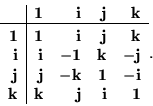
The multiplication table is

$$\begin{array}{r\vert rrrr} & {\bf 1}& {\bf i}& {\bf j}& {\b... ...}\\ {\bf k}& {\bf k}& {\bf j}& {\bf i}& {\bf 1} \end{array}.$$

The usual way of performing algebraic operations on these matrices is to write a sum such as 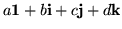$a {\bf 1}+ b {\bf i}+ c {\bf j}+ d {\bf k}$ in the form $s + {\bf v}$, where $s = a {\bf 1}$ and ${\bf v}$ is the rest of the sum. Doing that allows writing

$$( s + {\bf u}) ( t + {\bf v}) = s t + s {\bf v}+ t {\bf u}+ ( {\bf u}. {\bf v}) + ( {\bf u}\times {\bf v}),$$ (1)

particular interest attaching to the case where $s$ and $t$ are zero, leaving the product of two vectors to take the form of a scalar plus a vector. However, the inner (or dot) product is not the usual one, rather one with a MinkowskiMinkowski metric type metric:

$$\begin{eqnarray*} ({\bf u}\cdot {\bf v}) & = & - u_1 v_1 + u_2 v_2 + u_3 v_3, \... ...t[ \begin{array}{c} v_1 \\ v _2 \\ v_3 \end{array} \right]. \end{eqnarray*}$$

Since the inner product for a Minkowski metric can be positive, negative, or zero, taking it for the square of a norm requires considering the sign, unless an imaginary norm is acceptable. So to define the norm of a vector, use the absolute value of the metric, by setting

$$\begin{eqnarray*} \vert{\bf v}\vert & = & \surd{\rm abs}(({\bf v},{\bf v})), \end{eqnarray*}$$

note that it can vanish for a nonzero vector, and never forget the possible influence of the bypassed sign.

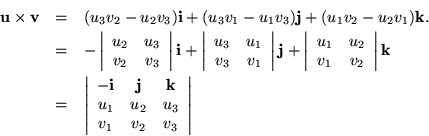
In turn the vector product differs slightly from its cartesian version. It is

$$\begin{eqnarray*} {\bf u}\times {\bf v}& = & (u_3 v_2 - u_2 v_3) {\bf i}+ (... ... u_1 & u_2 & u_3 \\ v_1 & v_2 & v_3 \end{array} \right\vert \end{eqnarray*}$$

The latter formula, almost traditional, abuses determinantal notation. But this particular formula never implies any multiplication of quaternions, so it works out well enough, although differing from the classical formula in the sign of the term associated with ${\bf i}$.