The evolution of an automaton can be described in matrix form, as well
as by the evolution function ![]() . The matrix required has to be
rectangular, since there are boundary cells at the ends of the string
whose evolution cannot be computed from the information available in
the string itself. The simplest matrix in the series describes the
cells of the second generation in terms of the cells comprising their
neighborhoods; two values
. The matrix required has to be
rectangular, since there are boundary cells at the ends of the string
whose evolution cannot be computed from the information available in
the string itself. The simplest matrix in the series describes the
cells of the second generation in terms of the cells comprising their
neighborhoods; two values ![]() can evolve from eight neighborhoods
{000, 001, 010, 010, 011, 100, 101, 110, 111}, so the
required matrix has the dimension
can evolve from eight neighborhoods
{000, 001, 010, 010, 011, 100, 101, 110, 111}, so the
required matrix has the dimension ![]() ; for Rule 22 it would take
the form:
; for Rule 22 it would take
the form:
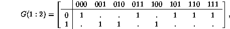
where the evident formula for the matrix elements is
![]()
Since the matrix is not square, successive generations of the evolution
cannot be obtained by raising it to powers. However, by iterating
![]() it is possible to obtain the matrix for further generations,
and thus to relate any pair of generations. Unfortunately such a procedure
corresponds to none of the commonly recognized operations on
matrices (such as the tensor product).
it is possible to obtain the matrix for further generations,
and thus to relate any pair of generations. Unfortunately such a procedure
corresponds to none of the commonly recognized operations on
matrices (such as the tensor product).
For example, we might work out, again for Rule 22, the matrix for one generation of evolution of the five-cell neighborhoods which will produce the three-cell neighborhoods which evolve into single cells. Such a matrix would be
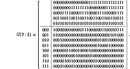
and finally, going one step further,
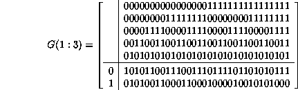
.
According to this scheme, one has ![]() , and a clear
procedure for advancing through further generations. Since the
dimension of these matrices increases rapidly -- doubling each
generation -- and since they have very few non-zero elements, they are
of more interest for theoretical discussions than as a practical means
of computation. In keeping with the fact that they represent a
function, there is exactly one non-zero element in each column, but
since they are not square, some rows must necessarily have several
non-zero elements. The exact distribution will vary from rule to rule
and to a great extent will characterize the rule involved.
, and a clear
procedure for advancing through further generations. Since the
dimension of these matrices increases rapidly -- doubling each
generation -- and since they have very few non-zero elements, they are
of more interest for theoretical discussions than as a practical means
of computation. In keeping with the fact that they represent a
function, there is exactly one non-zero element in each column, but
since they are not square, some rows must necessarily have several
non-zero elements. The exact distribution will vary from rule to rule
and to a great extent will characterize the rule involved.