solving second order equations

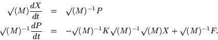
A second order version of the inhomogeneous system which has just been solved, suitable for a chain of particles, would read

$$\begin{eqnarray*} M \frac{d^2X}{dt^2} & = & - K X + F. \end{eqnarray*}$$

It should be turned into a pair of first order systems by inventing momenta (mass times velocity), but splitting the mass coefficient in the interests of having a symmetrical dynamical matrix to diagonalize later on:.

$$\begin{eqnarray*} \surd(M) \frac{dX}{dt} & = & \surd(M)^{-1} P \\ \surd(M)^{-... ... - \surd(M)^{-1} K \surd(M)^{-1} \surd(M) X + \surd(M)^{-1} F. \end{eqnarray*}$$

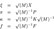
For the sake of not writing so many mass radicals, weighted coordinates and momenta could be introduced, and the elastic matrix replaced by a dynamical matrix. The forcing term might as well be adjusted too. So define:

$$\begin{eqnarray*} \xi & = & \surd(M) X \\ \pi & = & \surd(M)^{-1} P \\ \kap... ... = & \surd(M)^{-1} K \surd(M)^{-1} \\ f & = & \surd(M)^{-1} F \end{eqnarray*}$$

to have the pair of systems of equations summarized in one matrix equation,

$$\begin{eqnarray*} \frac{d}{dt} \left[ \begin{array}{c} \pi \\ \xi \end{arra... ...ght] + \left[ \begin{array}{c} f \\ 0 \end{array} \right] \end{eqnarray*}$$

The coefficient matrix is a matrix of constants, so the solution of the homogeneous equation is a matrix exponential. Furthermore, since

$$\begin{eqnarray*} \left[ \begin{array}{cc} 0 & - \kappa \\ 1 & 0 \end{arr... ...ay}{cc} - \kappa & 0 \\ 0 & - \kappa \end{array} \right], \end{eqnarray*}$$

there ia an Euler's formula

$$\begin{eqnarray*} \exp(\left[ \begin{array}{cc} 0 & - \kappa \\ 1 & 0 \en... ...sin(\surd\kappa t) & \cos(\surd\kappa t) \end{array} \right]. \end{eqnarray*}$$

Note that since $\kappa$ is a matrix, it could only invite misunderstandings to write $1/\surd\kappa$ instead of $\surd\kappa^{-1}$ in these formulas.

Turning at last to the inhomogeneous term, the overall solution is

$$\begin{eqnarray*} \left[ \begin{array}{c} \pi(t) \\ \xi(t) \end{array} \rig... ...gin{array}{c} f(\sigma) \\ 0 \end{array} \right] d\sigma}. \end{eqnarray*}$$

The integral, which makes a sine or cosine transform of the forcing function, has various interpretations, one of which is that it reduces all the accumulated forces to equivalent initial conditions which then modify the stated initial conditions propagate the result up to time t. The forcing function can be a pulse, a function of limited duration, or a permanent influence. Supposing the latter to be a harmonic force, say a sine or cosine itself, the phenomonon of resonance makes its appearance. Assuming that $\kappa$ were diagonal, there would be a series of scalar (really, 2x2) equations saying (putting $\surd\kappa = \omega_0$ and $f = \sin(\omega t)$)

$$\begin{eqnarray*} \xi(t) & = & {\rm initial value} + \frac{1}{\omega_0} \int_... ...+ \omega)\sigma)} {2\omega_0 (\omega_0 + \omega)} \right] _0^t \end{eqnarray*}$$

Given that $\omega_0$ is (the square root of) an eigenvalue, and that its provenance from a square root could endow it with either sign, one of the two terms will have a zero denominator whenever the forcing frequency coincides with $\omega_0$. No doubt physicists and engineers first became aware of eigenvalues on account of this circumstance. Although the denominator could be zero, that does not mean that the amplitude is immediately infinite, only that it will build up without limit. The integral with $\omega = \omega_0$ has a constant integrand, and the amplitude will build linearly at first, giving the zero denominator time to take effect.

In practice, a mechanical system would have friction, which would render $\omega_0$ complex, so resonances could be large without becoming infinite. Equivalently, the exciting force could be damped, with an implicit complex $\omega$, so the excitation would never last long enough to build up to an extreme amplitude.