Diatomic string

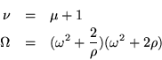
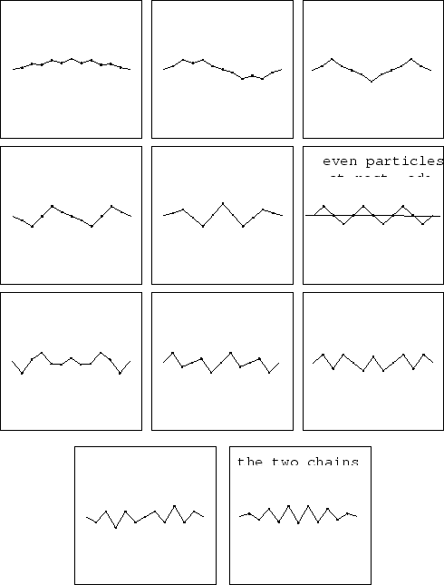
In a diatomic chain, two different kinds of particles are supposed, but they alternate with one another rather than having similar particles grouped together in sequence. The effect remains the interaction of one group with the other, but now that they are interspersed, the consideration has to be the even numbered particles competing with the odd numbered particles.

Figure: heavy and light particles alternate

The dynamical matrix would look like:

$$\begin{eqnarray*} A & = & \left[ \begin{array}{cccccc} \frac{-2k}{m} & \fra... ...urd(m M)} & . \\ . & . & . & . & . & . \end{array} \right]. \end{eqnarray*}$$

Introducing a mass ratio $\rho = \surd(M/m)$ and writing the common factor $k/\surd(Mm)$ outside the matrix gives the dynamical matrix a better appearance:

$$\begin{eqnarray*} A & = & \frac{k}{\surd(Mm)}\left[ \begin{array}{cccccc} -... ...\rho} & 1 & . \\ . & . & . & . & . & . \end{array} \right]. \end{eqnarray*}$$

Mathematically, what could be done is to combine a consecutive pair into a single unit cell by multiplying their wave matrices, and then raising this product to a power. Depending on whether the chain is of even or odd length overall, a single wave matrix may have to be incorporated to finish off the full chain. Although the dispersion relation for a single cell has to be more complicated, the advantage of constant wave numbers irrespective of the number of unit cells remains.

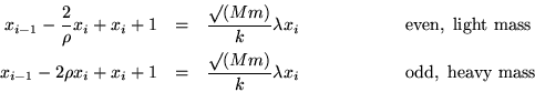
The eigenvalue equation for this matrix gives even and odd recursion equations,

$$\begin{eqnarray*} x_{i-1} - \frac{2}{\rho} x_i + x_i+1 & = & \frac{\surd(Mm)}... ...c{\surd(Mm)}{k}\lambda x_i \hspace{6em} {\rm odd,\ heavy\ mass} \end{eqnarray*}$$

Note that the geometric mean of the masses is a factor of $\lambda$ in both equations. To avoid square roots, introduce

$$\begin{eqnarray*} \omega^2 & = & \frac{\surd(Mm)}{k}\lambda \end{eqnarray*}$$

and two wave matrices,

$$\begin{eqnarray*} \left[ \begin{array}{cc} \omega^2 + \frac{2}{\rho} & -1 \\ ... ...& -1 \\ 1 & 0 \end{array} \right] & & {\rm odd,\ heavy\ mass} \end{eqnarray*}$$

Individually, they define dispersion relations similar to those for the uniform chain, but here it is necessary to evaluate their alternating products, taking into account that they do not commute unless $\rho = 1$.

$$\begin{eqnarray*} \left[ \begin{array}{cc} \omega^2 + \frac{2}{\rho} & -1 \\ ... ...rac{2}{\rho}) \\ \omega^2 + 2 \rho & -1 \end{array} \right]. \end{eqnarray*}$$

By symmetry, changing the order of the product would exchange the skewdiagonal elements. Recalling that $AB$ has the same eigenvalues as $BA$, the dispersion relation is the same for either product, namely

$$\begin{eqnarray*} (\omega^2+\frac{2}{\rho})(\omega^2+2\rho)-1-\mu)(-1-\mu) + (\omega^2+\frac{2}{\rho})(\omega^2+2\rho) & = & 0 \end{eqnarray*}$$

Introduce more abbreviations,

$$\begin{eqnarray*} \nu & = & \mu + 1 \\ \Omega & = & (\omega^2+\frac{2}{\rho})(\omega^2+2\rho) \end{eqnarray*}$$

to get the sequence

$$\begin{eqnarray*} (\Omega - \nu)(-\nu) + \Omega & = & 0 \\ \Omega \nu + \nu^2... ...\ & = & \mu + 2 + \frac{1}{\mu} \\ & = & 4 \cosh^2(\varphi). \end{eqnarray*}$$

So the calculation of $\Omega$ goes pretty much as usual. To get $\omega$ out of $\Omega$ is the interesting part; to simplify formulas still further, define $\alpha = \rho + 1/\rho$.

$$\begin{eqnarray*} \Omega & = & \omega^4 + 2 \omega^2\alpha + 4 \\ \omega^2 & ... ...ega))}{2} \\ & = & -\alpha\pm\surd(\alpha^2+4\sinh^2(\varphi)) \end{eqnarray*}$$

$$\begin{eqnarray*} \left[ \begin{array}{cc} \frac{\lambda + a + c}{c} & - \fra... ...c} & - \frac{c}{b} \\ 1 & - \frac{c}{b} \end{array} \right] \end{eqnarray*}$$

What really counts is whether $\sinh(\varphi)$ has to be imaginary or complex, which is best seen by yet another reformulation of the dispersion relation.

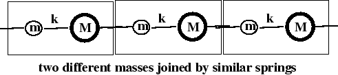
Figure: heavy and light particles alternate