


Next: Numerical integration with graphical
Up: Resonance in the Dirac
Previous: The Dirac equation
All in all, the Dirac harmonic oscillator is a good place to study resonances, especially if much smaller masses are considered than the ones which characterize the actual experience of physicists. Of course, that makes a comparison with experiment correspondingly difficult.
The one-dimensional Dirac equation for a particle of rest mass m0 has a matrix form
 |
= |
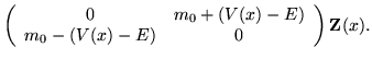 |
(1) |
The substitutions
lead to a convenient solution matrix,
 |
= |
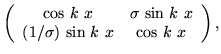 |
(2) |
but only for a constant energy difference E - V, and for real k. Formally the result holds for immaginary k but in that case, a classically forbidden region, it is preferable to redefine both k and  to make them real and then use hyperbolic functions.
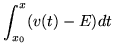
There are other approximations which are useful; for example when the mass is small enough to be neglected, the coefficient matrix is antisymmetric. Setting
 |
= |
 |
(3) |
the solution becomes
|
= |
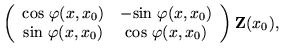 |
(4) |
which is a pure rotation in the phase plane.
There is a standard procedure for correcting an approximate coefficient matrix in a system of differential equations. Suppose that the full coefficient M is
split into a sum
wherein A is the convenient approximation and B is a correction, not necessarily small. All kinds of splittings are possible: symmetric and antisymmetric parts, averages and deviations, large and small components, to mention three.
Supposing that the auxiliary equation
 |
= |
 |
(6) |
has already been solved subject to the initial condition
 ,
and that we intend to write
,
and that we intend to write
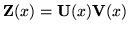 ,
we find that
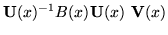
,
we find that
 must solve the differential equation
 |
= |
 |
(7) |
subject to the same initial condition as  .
.
Next: Numerical integration with graphical
Up: Resonance in the Dirac
Previous: The Dirac equation
Microcomputadoras
2001-01-09