 |
Given the assumption that the ether is going to be the background against which glider theory is to be developed, their velocities can be read off as slopes of the fault lines in the ether lattice. That does not mean that there are not other lattices which admit gliders. We have searched for them and found several. One of them, with T5's, plays a role in Cook's extensible gliders, namely the E and the G series. We have tentatively called it an ![]() tile. However, observations of evolution from random initial conditions show that the ether lattice is overwhelmingly, if not exclusively, favored. So that is the environment in which the potentialities for gliders should be examined.
tile. However, observations of evolution from random initial conditions show that the ether lattice is overwhelmingly, if not exclusively, favored. So that is the environment in which the potentialities for gliders should be examined.
It is worth emphasizing the subjectivity of the concept of a glider. Originally, in Conway's formulation of Life, they were recognizable discrete objects which moved against a quiescent background. In fact, the name ``glider'' reflects a peculiarity of that movement, that the object flipped about its line of motion as it progressed, reminiscent of glide planes in crystallography. Here there is no flipping, and the background is not quiescent, but those are quibbles.
Gliders find their place in de Bruijn diagrams given two or more cycles mutually interconnected. The pattern of one of them can be embedded in an environment created by the other; in Life one of those cycles is the self-loop of the quiescent node. If the connection is unidirectional, space is split in half rather than embedding; the structures are called fuses. If the two cycles are disconnected, there are two distinct patterns which cannot coexist shift-periodically.
Which is the glider and which is the background, and whether a thing is called a glider at all, dependends on appearance and aesthetics.
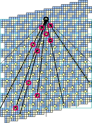
Figure 13 shows the fault lines in the ether lattice. On general principles, superluminal gliders are excluded, but not all the remaining possibilities turn out to be realized. Those whose de Bruijn diagrams are accessible to our computational facilities show the presence of only those which Cook announced. The absence of others depends on the lack of interconnection of configurations of the given shift periodicity to the subsets of the ether lattice having the same specifications.
There are selection rules; for example, nothing speedier than Cook's A and B gliders. Showing this has been set forth as a challange, but it is empirically true that the larger the largest triangle in a glider, the slower it moves. Slowness is related to the problem of filling the areas under the hypotenuses when large triangles are strung alongside each other. The triangle, the further down its next occurrence is likely to be found, promoting lethargy.
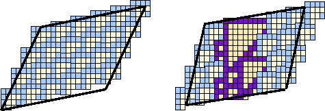 |
Figure 14 shows a unit cell for one of Cook's E-gliders, which shifts left by 4 every 15 generations. The unit cell looks to be
![]() ,
the height being the period and the width being the distance necessary to resynchronize the ether lattice. However, the actual figure is
,
the height being the period and the width being the distance necessary to resynchronize the ether lattice. However, the actual figure is
![]() because the unit cell is a rhombus, so the dimensions cited are sections, not altitudes.
because the unit cell is a rhombus, so the dimensions cited are sections, not altitudes.
To reconcile the unit cell of 285 cells with tiles which it contains, consider
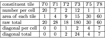
Summing the areas of the tiles gives 336 cells. There are 23 tiles altogether with 37 diagonal cells, each of which has been covered twice in this accounting. The net total of 299 factors into
![]() ,
which is the area of the unit cell. The factors relate to the dimensions of the cell which, as a rhombus, has an effective height and an effective width.
,
which is the area of the unit cell. The factors relate to the dimensions of the cell which, as a rhombus, has an effective height and an effective width.