Commentary on Andrew Wuensche and Mike Lesser's new book, ``The Global Dynamics of Cellular Automata.'' Addison-Wesley, 1992 (ISBN 0-201-55740-1) continues. We have digressed into some issues of matrix theory and graph theory in the expectation that a better understanding of the foundations of cellular automaton theory will help with understanding some of the topics of the book, such as Langton's parameter, Z, and perturbations (mutations).
To maintain a connection with the book, consider again the A and B matrices for Wolfram's (2,1) Rule 22:

For a chain of three cells, we have eight products of these three matrices, corresponding to the ancestors of 000, 001, 010, and so on:
0.15em

0.15em

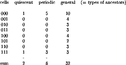
From these matrices we draw conclusions about the number of ancestors by looking at the (0,0) elements (quiescent-at-infinity configurations), traces (periodic configurations) or summing all the elements in the matrix (unrestricted configurations):

Turning to page 96 of the Atlas, we confirm that s=8 (sum of the ``periodic'' column) and mp=5 (largest number in the ``periodic'' column). The only branching ratios are 3 and 5 (and of course, 0), confirmed by examining the diagram at level 3. The fact that g=6 (GOE configurations) follows from the fact that six of the matrices have zero diagonal, and hence trace zero.
None of the matrices is identically zero, so there are no poison words of length 3; however, the fact that the multiplicities are not uniform goes against the theorem (not yet discussed) about nonuniform multiplicities implying a Garden of Eden.
These details relate to a tiny fraction of the information contained in the Atlas, but they should suffice to establish the fact that as long as one is prepared to multiply A and B matrices, several different types of ancestors can be counted. Also, if one is prepared to work with symbolic matrices rather than numerical matrices, quite explicit ancestors can be calculated.
Of course, what is really wanted are general theorems about the matrices, so that all their products DON'T have to be calculated explicitly.
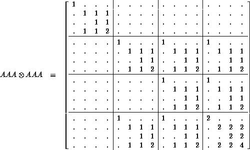
Considerable space would be consumed by listing all eight tensor squares, but the next point can probably be made with just one of them: small

Note the following comparisons:

In each case, the corresponding quantity is squared in the tensor square. Examining the structure of the matrix, it isn't hard to see why. However, this should give a graphic illustration of why the tensor powers participate in the calculation of moments, and how the tensor square (the connectivity matrix of the pair diagram) will eventually be involved in calculating the variance. Note that if we want to establish zero variance, it is only necessary to compare the square of the first moment with the second moment.
What is needed is ![]() ; when the power is expanded
and all the terms collected, one finds one term for the square of the number
of ancestors of each configuration. To get the third moment, take
; when the power is expanded
and all the terms collected, one finds one term for the square of the number
of ancestors of each configuration. To get the third moment, take
![]() , whereas if there were three
states, there would be a C matrix, with a second moment expressed in terms
of
, whereas if there were three
states, there would be a C matrix, with a second moment expressed in terms
of ![]() , and so on.
, and so on.
Because of the powers, we are interested in the rate of growth of the terms in parentheses in the last paragraph, which boils down to finding their largest eigenvalues or more generally, finding estimates or bounds for them.
More commentary will follow.