Commentary on Andrew Wuensche and Mike Lesser's new book, ``The Global Dynamics of Cellular Automata.'' Addison-Wesley, 1992 (ISBN 0-201-55740-1) continues. For the moment we are laying a groundwork of matrix and graph theory, rather than discussing the book explicitly; reference to the book will still provide examples for statements which will be made.
Much of the theory of cellular automata, and especially of one dimensional cellular automata, can be described with the aid of de Bruijn diagrams and their associated connectivity matrices. The calculation of ancestors (for a binary automaton) can be accomplished by using a pair of these matrices, one for each of the two states into which a neighborhood can evolve.
To write down a de Bruijn matrix quickly, and to interpret one rapidly, use Wolfram's scheme for enumerating automata. Suppose that the rule is
![]()
The corresponding positions in the connectivity matrix are

where all elements marked by dots are filled with zeroes. The length of the ``steps'' in the matrix correspond to the number of states in the automaton, while the number of steps reflects the size of the neighborhood, as does the number of ``flights of stairs;'' the two are always equal.
Large de Bruijn diagrams are hard to draw, having so many nodes and links. The best visualization we have found is just to draw a circle, divide the circumference into the requisite number of nodes, and treat them as though they were k-adic numbers modulo the total number of start strings. All but the simplest are still quite congested. Artistically, they have a pleasing structure.
From the basic de Bruijn diagram, others may be derived. One is the subset diagram, whose elements are subsets of nodes from the primitive diagram. the concept was introduced in the 1950's by E. L. Moore, who was interested in experiments which could identify the state of an automaton, or to place it in an arbitrarily prescribed state. Its relation to calculating ancestors is a consequence of offering a sure and easy way to ascertain whether the primitive diagram contains a given path or not.
To create a subset diagram, link two nodes if there is a link from at least one node in the source (tail) subset to all the nodes in the destination (head) subset. Or in other words, take a source subset and run through all the nodes to which its members are linked; that collection is the destination. When there are no such links, the subset is connected to the empty set. That way a uniform quota of links is guaranteed for each node in the subset diagram, so that arbitrary paths can always be found; but getting trapped at the empty set is always a possibility.
With respect to ancestors, not caring about the start string means beginning at the full set. Any path leading from there to the empty set implies the lack of an ancestor, and thus a non-empty Garden of Eden. Many conclusions can be drawn, for example, the shortest ancestorless string, the longest loopless string with ancestors, and so on. And, of course, if there is no path at all, there is no Garden of Eden.
Since the subset diagram is naturally ordered, not finding a Garden of Eden
leads to some natural questions: what is the largest set that still leads
to the null set? what is the smallest set still reachable from the full
set? and so on. G. A. Hedlund![]() and his followers have studied these questions in much
detail.
and his followers have studied these questions in much
detail.
Although the subset diagram reveals the existence of ancestors, it is not very helpful in identifying them, because it is not so easy to backtrack.
For Wolfram's (2,1) Rule 22, the subset diagram has 16 elements, which we may rank by size from the full set to the empty set.
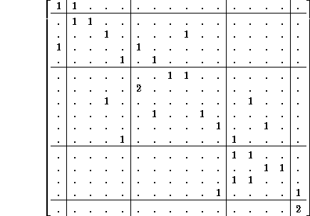
Connection matrix:

Noteworthy details: The 4x4 unit-class submatrix in the lower right hand corner is almost a de Bruijn diagram, because most of its nodes have continuations with either a 0 or a 1, but the start string 11 leads to both 110 and 111 to form a neighborhood which evolves to 0, so it links to a two-element subset via 0 and the empty set via 1. That explains the next-to-last row. This is also the only direct linkage to the empty set in the matrix.
In fact, the eighth is the smallest power of the matrix with a direct link from the full set to the empty set, corresponding to the ``poison word'' 10101001 (and of course, its reflection, 10010101). This is easier to appreciate by drawing the diagram, without a computer program which can display the matrix and its powers. For any Rule, by the 16th power, a decision will necessarily have been reached, as to whether the (full, empty) matrix element is zero or not. (But, the de Bruijn diagram only had 4 nodes)
Primitive diagrams have another kind of derivative, the pair diagram (and more generally, the n-tuple diagram); both ordered pairs and unordered pairs may be considered. Consider ordered pairs; (x,y) is linked to (X,Y) if x is linked to X AND y is linked to Y. A pair diagram is a kind of greatest lower bound between its constituents (a greatest common denominator, if you wish). Unordered pairs might be more convenient if both members were taken from the same set, such pairs are also subsets.
The most evident application of a pair diagram lies in testing whether or not the same sequence of nodes can be found in two different places in the primitive diagram, and therefore is related to establishing uniqueness. If two paths exist, lay them out side by side, pair their corresponding links, and get the path in the pair diagram. Conversely, any path in the pair diagram may be decomposed into its constituents.
A more subtle application of the pair matrix lies in calculating variance. If the powers of the connection matrix of a graph reveal the number of paths of the corresponding length between nodes, then the powers of the pair matrix reveal the square of this number, or in other words, the second moment. From there to the variance is an exercise in elementary statistics. The application to counting ancestors lies in the observation that if some configurations have more ancestors, then others have fewer, which must result in a non-zero variance. Still, the connection is not easy to prove.
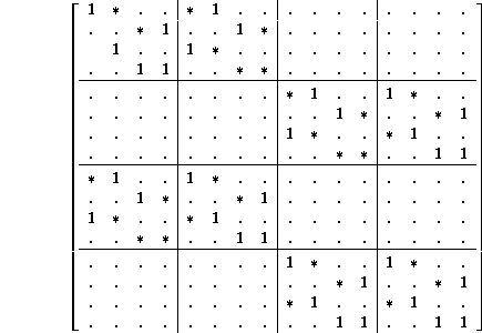
For Wolfram's (2,1) Rule 22, the pair diagram has 16 elements, thus a 16x16 connection matrix,

Stars designate locations where 1's could appear, but don't, in Rule 22. Note how the structure of the tensor product makes the overall matrix look like a de Bruijn diagram, as well as each submatrix. There are better arrangements of the nodes, and consequently of the indices; Wuensche and Lesser's clustering techniques ought to be followed more closely. That is, the complementary automaton is lurking in this matrix, if one only knows how to perceive it.
More commentary will follow.