Mandelbrot set for second degree polynomials

Linear mappings and fractional linear mappings have the structure which we have already seen. The next most complicated, in terms of polynomial degree and hence in number of fixed points and their stability, are quadratic mappings:

P(z) = az²+bz+c. (100)

However, the use of a scale factor and shift of origin can transform any quadratic polynomial to the form

w = z²+c. (101)

which depends on one single complex parameter. The fixed points are

z = z²+c (102)

$$\frac{1\pm\surd(1-4c)}{2}.$$ z = (103)

at which the derivatives are 2z, or

$$= 1\pm\surd(1-4c).$$ w' (104)

Unless $c = \frac{1}{4}$, where the fixed points are both neutral, one is stable, the other unstable (or maybe both are unstable).

The critical points are where

w' = 2z = 0.

so there is just one, at the origin.

Counterimages satisfy

w = z²+c (105)

$$\pm\surd(w-c)$$ z = (106)

and so are negatives of one another (as is evident from the defining equation).

Since everything depends on this one number, c, consider values for which the fixed points can be neutral, the dividing line between stability and instability. There set $w'=e^{i\phi}$:

$$e^{i\phi} 1\pm \surd(1-4c)$$ = (107)

$$(e^{i\phi}-1)^2$$ = 1-4c (108)

$$\frac{1}{4}\left(1 - (e^{i\phi} - 1)^2\right)$$ c = (109)

$$\frac{1}{4}(1 - e^{2i\phi} + 2e^{i\phi} - 1)$$ = (110)

$$\frac{1}{4}(2e^{i\phi}-e^{2i\phi})$$ = (111)

This is the sum of two contrarotating vectors, one double the length of the other and the shorter spinning at twice the angular velocity.

The figure is a cardioid, the interior of which contains values of c for which there is a stable fixed point.

Passing to the iterated function,

w = (z²+c)²+c (112)

= z⁴ + 2cz² + c² + c, (113)

and using long division,

z⁴ + 2cz² + c² + c = (z²-z+c)(z²+z+(c+1)), (114)

so the iterate still has the fixed points of the primitive function, and two more besides, which are:

$$\frac{-1\pm\surd(1-4(c+1)}{2}$$ z_f = (115)

To get the stability of the iterate, we need its derivative

w' = 4z(z²+c) (116)

at the new fixed points, where

z² + c = -(z+1) (117)

z² + z = -(c+1). (118)

That results, in sequence, in

w_f' = -4z_f(z_f+1) (119)

= 4(c+1). (120)

To get the contour of neutrality this derivative must have modulus 1, leaving

$$-1 + \frac{1}{4}e^{i\phi}$$ c = (121)

which is a circle at center -1, radius $\frac{1}{4}$, which has to be joined with the previous cardioid. It extends leftward to $-\frac{3}{4}$, so they are tangent.

All this calculation can be repeated for longer and longer cycles, although the algebra becomes ever more intricate and quickly lies beyond solution by formula.

The locus of stability can be located by more direct numerical processes, and in its totality forms the boundary of the Mandelbrot set. The higher loci will still resemble cardioids or circles, although they interfere with one another sufficiently that none of them will have that exact form although approximating it recognizably.

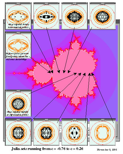
The Mandelbrot set is a map describing the stability of the fixed points and cycles of w = z²+c, in terms of the single complex parameter c. Because the results can be shown visually on a single sheet of paper, this function has been a popular one to study. Of course, other functions could be studied by the same procedure, without a corresponding graphical visualization, although the term ``Mandelbrot set'' could still be used.

Also bear in mind that each point in the Mandlebrot plane represents a different complex function, whose values and the values of whose iterates can also be graphed on a sheet of paper. The contours for high iterates of z²+c show a step function which jumps from one value to another at points which are members of the Julia set. The number of steps depends on the location of c within the Mandelbrot set, but more precisely in which of the little bubbles it lies.

Figure 10 contains an image of the Mandelbrot set, surrounded by a sequence of insets showing the behavior of the iterates of w = z²+c for some values of c lying along the real axis. Of coures, when c=0, which sits at the center of the stable cardioid, the figure is a parabola, flattening more and more inside the unit circle, while rising more and more rapidly outside.

The vignettes show the effect of iteration backwards, since the contours have been produced by computing counterimages of a small circle surrounding the origin. Correspondingly, a ``small'' circle surrounding infinity, |z|=2 has been counterimaged to produce a series of contours approaching the Julia set from the outside.

It might have been better if the circle surrounding 0 had surrounded the stable fixed point instead, but this version reveals some interesting aspects of the mapping process. The counterimage depends on a square root and degenerates when the argument of the square root vanishes, which is when the radius of the circle reaches the absolute value of c. Up to that point, the circle deforms into ellipses and figures with additional Fourier components, but then a critical point has been reached where the counterimage lacks definition. Beyond that value the circle splits into two components, and then it may split further as additional critical points are encountered.

In any event, the expanding counterimages approach the Julia set from the inside, which has to be confined between the two sequences of counterimages, approaching from the inside and from the outside. Of course, there may not be an ``inside,'' as would happen outside the Mandelbrot set, with both finite fixed points unstable.

  

Figure 10: A survey of points in the Mandelbrot set, showing their corresponding Julia sets.

Creating a polynomial with certain fixed points is just the same as creating a polynomial with particular zeroes: write

$$(z-f_1)(z-f_2)\ldots(z-f_n) + z.$$ P(z) = (122)

When that is done, the derivatives have all been assigned, because

$$1+\sum_j\prod_{{\rm omit}\ j}(z-f_j)$$ P'(z) = (123)

$$1 + \prod_{{\rm omit}\ i}(f_i-f_j).$$ P'(f_i) = (124)

Some ingenuity could be exercised in setting aside one of the fixed points and moving it around to get a desired derivative at some other fixed point, but a better way to make a certain fixed point have a desired modulus of stability would be to use Hermite interpolation. For polynomials of even degree, any derivatives at all can be given to half of the data, the other half being the actual locations of the fixed points.

There is a precaution to be observed when passing between zeroes and fixed points in describing a polynomial. Infinity is not a zero of a polynomial because the dominant term will always increase towards infinity, even though the analysis of an essential singularity may lead to such a zero; think of $\exp(-\infty)$. On the other hand, infinity is a fixed point for polynomials, at least on the Riemann sphere where there is only one infinity.

The precaution consists in counting fixed points accurately; a polynomial of degree d has exactly d zeroes, and apparently d fixed points. But the number is actually d+1 because of having to include infinity.