Mathieu functions

One of the easiest ways to get a differential equation with periodic coefficients is to insert a sine or cosine in place of the frequency in the equation for simple harmonic motion; with stylized symbols, the result is Mathieu's equation:

$$\frac{d^2}{dx^2}Y + (a-2q\cos(2x))Y$$ = 0 (326)

The outstanding new feature in such an equation is the possibility that there will be periodic solutions to match the periodic coefficient, but we already know that that is not to be expected. Rather, although some solutions may be periodic, the result of a translation through a single period will be to form a specific linear combination of solutions which will be reapplied for any further translations.

  

Figure 18: stability chart for solutions to the Mathieu equation.

The quantities of interest are then the eigenvalues and eigenvectors of the period matrix. Unless an eigenvalue is exactly equal to 1, there will be no strictly periodic solution, but the failure reduces to a multiplying factor, which is the eigenvalue. The eigenvalue -1 is exceptional, for implying subperiodic solutions -- those which repeat having skipped a unit cell rather than immediately. The main feature of qualitative interest is the absolute value of the eigenvalues, which describes the rate of growth of solutions with respect to the translational lattice.

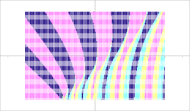
There are two parameters in the Mathieu equation, a multiplier a which would be an energy level in a quantum mechanical equation, and an intensity q. The main item of interest in the equation is often its stability chart, rather than the exact solutions themselves. The stability chart is a contour plot of the absolute value of the eigenvectors of the period matrix as a function of the two parameters a and q. Given that the solution matrix of the equation is unimodular, half its trace is the cosine of the logarithm of the eigenvalue. Therefore plotting the trace gives the required information, relative to the values 1 and -1. Contours are more informative than absolute values because all the quantities in the discussion are real and signs can be retained.

Figure 18 is just such a contour plot, although it bears some explanation. For q=0 the equation reduces to the harmonic oscillator, a being the square of the frequency. When a is positive, the solutions are trigonometric, when a is negative, they are hyperbolic. The place where a=0 is slightly off center, to the left. Half the trace of the period matrix is $\cos(\surd a\ s)$, whose own period is $2\pi/\surd a$ and therefore whose contour values will reach $\pm 1$ at ever lengthening intervals. The thickness of the contour bands along the axis at the lower margin is an artifact caused by the horizontal tangents of the cosine at those points.

Along the line where a=2q, the amplitude of the cosine matches the harmonic oscillator parameter; quantum mechanically that would be a classical turning point, with the solution matrix taking the Jordan normal form; classically the same anomaly just gets a different interpretation. Visually, the line separates the region where the hyperbolic solutions represent a narrow intrusion into a region of essentially periodic solutions, and the reverse. In the outer region, hyperbolic solutions are the norm, oscillatory solutions requiring narrowly defined parameter ranges for their existence.

A much more detailled analysis of the Mathieu equation and periodic potentials in general can be found in course notes [22].