Dirac harmonic oscillator

As an example of a one-dimensional Dirac equation, consider the harmonic oscillator with potential $\frac{1}{2}x^2$ and mass m

$$\frac{d}{dx} \left[\begin{array}{c} \phi(x) \\ \psi(x) \end{array}\right] \left[ \begin{array}{cc} 0 & m - E + \frac{1}{2}x^2 \\ m + E - \... ...nd{array} \right] \left[\begin{array}{c} \phi(x) \\ \psi(x) \end{array}\right]$$ = (336)

In normal physical problems with units compatible with atomic dimensions the mass is of the order 137, which completely dominates the equation. For mathematical purposes it is more convenient for the mass to be comparable to 1, although both extremes lead to illustrative partitions of the coefficient matrix. If the mass dominates, the solutions are hyperbolic functions, whereas they are completely trigonometric in nature when the mass is zero.

For moderate mass, the region ``inside'' the potential well gives oscillatory solutions, similar to the Hermite polynomials fount in the Schroedinger equation. In the ``mass shell'' the solutions are exponential, as expected. However there is a new feature of the Dirac equation, in the ``outside'' region the solutions are again trigonometric, although their phase advance with distance is opposite to the ``inside'' behavior. For particles in the actual physical world, the mass shell is very thick, becoming infinitely so as the nonrelativistic limit is approached.

  

Figure: wave functions for a Dirac harmonic oscillator. The potential varies with z² making the wave function resemble $\sin(z^3)$ and $\cos(z^3)$. An even function is shown, the two parabolas are matrix elements of the coefficient matrix, and delimit the mass shell.

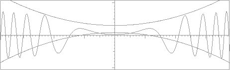Figure 21 shows a solution for an energy value that gives a very slight oscillation within the well, but oscillations with rapidly increasing frequency outside the well.

  

Figure 22: wave functions for a Dirac harmonic oscillator. Wave functions for a series of energies are shown in perspective view. The solutions are odd; gaps locate the classical turning points.

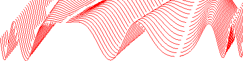Figure 22 shows a perspective view, with hidden line suppression, of a series of solutions over an energy range. The movement of the classical turning points can be seen, as well as the variation of frequency with energy. There is some jaggedness on acount of the relative large increment in the horizon function which suppresses hidden lines.

  

Figure 23: wave functions for a Dirac harmonic oscillator in the phase plane.

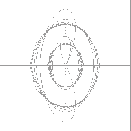
Figure 23 shows the solution of the Dirac harmonic oscillator in the phase plane. The solution consists of three sets of circles, connected by hyperbolic arcs. Two of them are superposed, by symmetry, representing the solution at large positive and large negative distances, respectively. As the energy varies, the ratio of the raduis of the inner circles to the outer circles will change; this is the quantum mechanical phenomonon of resonance and antiresonance. At resonance, the inner amplitude is a maximum relative to the asymptotic amplitude.

All one-dimensional Dirac equations afford an oportunity to split the mass term from the energy term, analogously to the WKB splitting already used for the Airy function. The kinetic energy term multiplies a unit antisymmetric matrix, so the solution is an Euler-formula exponential with an angle gotten by integrating the kinetic energy. For the Dirac harmonic oscillator, the angle is

$$\phi \int_0^x(E-\frac{1}{2}\sigma^2) d\sigma$$ = (337)

$$Ex +\frac{1}{6}x^3$$ = (338)

Accordingly the matrix U is $\exp(\phi {\bf i})$, the usual matrtix representing a rotation. But then the equation for the second factor, V has the coefficient

$$e^{-\phi {\bf i}} (m{\bf j})e^{\phi {\bf i}} m \left[\begin{array}{cc} \cos(2\phi) & \sin(2\phi) \\ \sin(2\phi) & -\cos(2\phi) \end{array}\right]$$ = (339)

corresponding to a rapidly spinning mirror.

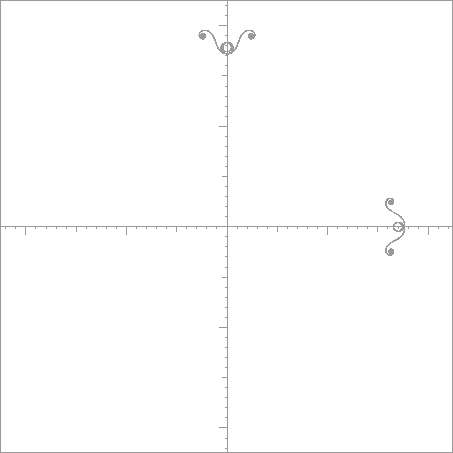
The solution for this coefficient is shown in Figure 24, whose most notable feature is the small asymptotic amplitude of oscillation of the solution. In the asymptotic region the mass, however large, is eventually dominated by the increasing potential energy, so the existence of mass or not is inconsequential. Near the origin, of course, the effects are more tangible. It is precisely in that region that the effects of resonance will be manifest.

  

Figure 24: Wave functions for a factorized Dirac harmonic oscillator. The massless solution is a rotation with argument proportional to z³. The factored equation adjusts for the mass.

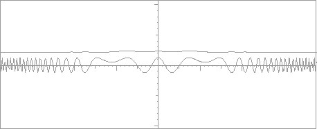Figure 25 shows these results more dramatically than the configuration space plots, and give some idea of the practical utility of the factorization. A much more detailled analysis of the Dirac Harmonic Oscillator can be found in course notes [21].

  

Figure 25: wave functions for a factorized Dirac harmonic oscillator in the phase plane.