Four-point two-dimensional approximation

Interpolation over triangles to get a linear approximation in two dimensions conflicts with the rectangular layout over a grid characteristic of most data sets, although the problem is readily resolved by splitting the rectangles into a pair of triangles.

Another approach to interpolating rectangular data is to use the cartesian product of coordinatewise linear interpolation. It has the further advantage that the corners of the coordinate rectangles can be the four interpolation points which the method requires.

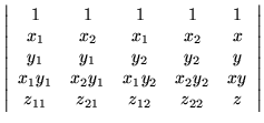
Consider the Vandermonde determinant

$$\left\vert \begin{array}{ccccc} 1 & 1 & 1 & 1 & 1 \\ x_1 & x_2 &... ... x_2 y_2 & xy \\ z_{11} & z_{21} & z_{12} & z_{22} & z \end{array} \right\vert$$ = 0. (35)

The weight matrix is a Kronecker product

$$\left[ \begin{array}{cccc} 1 & 1 & 1 & 1 \\ x_1 & x_2 & x_1 & x_... ...& y_1 & y_2 & y_2 \\ x_1 y_1 & x_2 y_1 & x_1 y_2 & x_2 y_2 \end{array} \right]$$ M = (36)

$$\left[ \begin{array}{cc} 1 & 1 \\ x_1 & x_2 \end{array} \right] \otimes \left[ \begin{array}{cc} 1 & 1 \\ y_1 & y_2 \end{array} \right]$$ = (37)

which therefore has the inverse

$$\frac{1}{x_2 - x_1} \left[ \begin{array}{cc} x_2 & -1 \\ -x_1 & ... ...}{y_2 - y_1} \left[ \begin{array}{cc} y_2 & -1 \\ -y_1 & 1 \end{array} \right]$$ M^-1 = (38)

$$\frac{1}{(y_2 - y_1)(x_2 - x_1)} \left[ \begin{array}{cccc} x_2 y... ... -x_2 y_1 & y_1 & x_2 & -1 \\ x_1 y_1 & - y_1 & - x_1 & 1 \end{array} \right]$$ = (39)

This time the interpolation formula z = Y^T M^-1 X uses the function values at the corners of the rectangle,

$$Y^T = \left[ z_{11}, z_{21}, z_{12}, z_{22} \right]$$

as a row of coefficients, with the variables {1, x, y, xy} constituting X. For purposes of contouring, however, the Vandermonde determinant would have been expanded differently, making use of a Laplace expansion according to the last column to get

A - B x + C y - D x y + E z = 0 (40)

and thence

$$y = - \frac{A - B x + E z}{C - D x}$$ (41)

The pole in this formula is nice because it is capable of accomodating a saddle point in the contours, although the formula will still have problems with maxima and minima.