Commentary related to Andrew Wuensche and Mike Lesser's book, ``The Global Dynamics of Cellular Automata.'' Addison-Wesley, 1992 (ISBN 0-201-55740-1) continues. Some observations on Langton's parameter, lambda, are in order.
We have described a 'Stastical Gerschgorin Theorem' (which is more of a formula than a theorem) which assigns a prominent role to the fraction of neighborhoods begetting each state in the enumeration of ancestors. These fractions enter into the calculation of moments with a correction term which experience shows to be small; if not always zero, its size is predictable and consistent.
If one calls such fractions 'Langton's parameter,' one has a solid basis for classifying automata according to such a parameter, whatever it is called. In other contexts, the fraction plays a role in calculating self-consistent probabilities, although there it yields a zero-order'th approximation to the fixed point.
As a predictor of automaton behavior, lambda has gained a mixed acceptance; Wuensche and Lesser introduce Z with the claim that it is a more sensitive indicator. The reason for this, among other things, is the bad company which Rules 18 and 126 are seen to be keeping in the example which follows. However, in browsing through an Atlas such as theirs, there is a tendency to see what one expects to see, particularly given the mass of data and their similarity to one another. So it behooves us to sharpen our tastes somewhat.
The situation may be likened to that prevailing in Botany before the advent of Carolus Linnaeus; there were tall trees and bushy trees and trees that kept their leaves through all seasons and those that shed their bark instead of their leaves, and those that smelled good and those that raccoons climbed in and others which monkeys preferred, and so on. Classifying them and every thing else according to the layout of their reproductive organs seemed rather prosaic, but in the end it brought order to a lot of chaos. And the monkeys even got to keep their tree (Araucaria araucana).
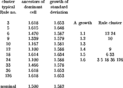
Calculating the average number of ancestors is like calculating the bushiness of our tree, in which case calculating their standard deviation amounts to observing whether this bushiness is strictly observed or whether it can vary considerably. Once again, examining a specific example may be helpful. Suppose lambda is 25% (lambda ratio = 0.5 in the Atlas). There are 56 (2,1) Rules with this ratio (including those with lambda = 75%), which the Atlas assigns to 11 clusters. The growth factors for the quiescent configuration and for the standard deviation in the number of ancestors are shown in the table below.

The histogram on the side gives an idea of how the growth factor of the A matrix, the column in the table titled 'ancestors ...,' are distributed around their mean of nominal value of 1.500. The other column has a parallel distribution.
The range 1.1 to 1.6 should be compared with the nominal values of 1.25 for ab=35 Rules and 1.75 for ab=17 Rules; if there is any transgression, it is for the Rules with small growth rates.
What we have to decide by looking at the Atlas is, whether this is all true, and whether, by knowing it, there are some features of the basins there displayed which should attract our attention, maybe even stand out.
(Has anyone noticed that in the Atlas, although the custom is to place the panel showing evolution from a single cell on the left and that from a random initial configuration on the right, this has been reversed for Rule 4 on page 88? Such are the delights of trying to publish an exceedingly detailed book and getting everything right)
Up until now, we have been unwilling to identify ``maximal growth rate'' with ``eigenvalue of A,'' because we have not proven rigorously that this is, in fact, the maximal growth rate. On the other hand, it is evident by inspection that the quiescent configuration will have the most ancestors, both according to the theory which has been presented in this series, and the empirical data comprising the Atlas; it only lacks a proof.
Another source of discrepancy is the fact that we have elaborated a general theory without boundary condition, whereas the Atlas is concerned exclusively with periodic configurations. Nevertheless, the nature of the general theory is such that all conclusions regarding multipliers, such as growth rates, apply equally to every variant of the boundary conditions which can be obtained by varying the metric matrix. This specifically includes periodic boundary conditions.
The one restraint which must be observed, is that it takes time for growth factors to reach the maximum eigenvalue of a matrix, so that conclusions should not be drawn for periodic configurations of a very short length. What constitutes 'very short' varies from Rule to Rule, but is closely related to the variation in size of the matrix elements within A, and especially to its pattern of zeroes.
One might wonder whether Garden of Eden configurations are included within this sweeping generalization, and the answer is yes, subject to the same precautions. The reason is that in a general automaton, poison words, and hence Gardens of Eden, arise because of incompatibilities - the requisite series of ancestral neighborhoods simply can't be found. In addition, likely ancestors may fail to meet boundary conditions.
For small rings, more ancestors will be lost because of boundary conditions. Recall that for Rule 22, eight is the shortest ring which has a poison word. But as rings grow longer, it is easier and easier to accommodate boundary conditions - two fragments which won't work separately may join together to compensate each other's deficiencies. Consequently for long rings, the Garden of Eden may be reduced by 1/4th, but otherwise its growth will follow that of the general theory.
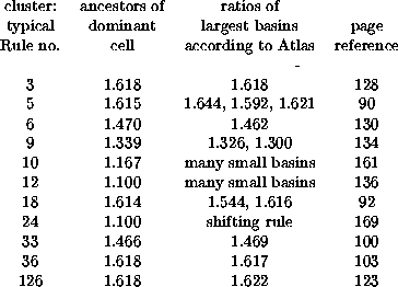
Returning to ``maximal growth rate'' and being willing to equate it with the larger of the dominant eigenvalues of the A, B pair (which implies that the quiescent configuration (or pair of alternating uniform configurations if none is quiescent, or uniform ancestor of the quiescent configuration when the dominant eigenvalue does not belong to the latter), we could compare growth and eigenvalue for the 26 (lambda ratio = 0.5) clusters:

Except for three clusters with many small basins, the agreement is
exemplary![]() .
.
More commentary will follow.