Commentary on Andrew Wuensche and Mike Lesser's new book, ``The Global Dynamics of Cellular Automata.'' Addison-Wesley, 1992 (ISBN 0-201-55740-1) continues. We have discussed how to form a de Bruijn diagram for a cellular automaton rule, its connectivity matrix, and how evolution splits the matrix into submatrices, which can be used to count ancestors. The rows and columns of the de Bruijn matrix are labelled by Wuensche and Lersser's ``start strings,'' but the columns are really ``stop strings.''
To fix ideas, consider the two matrices for Wolfram's (2,1) Rule 252, which is associated with rules 3, 17, 63, 119, 238, 192, and 236 in the Atlas, on pages 128 and 129.
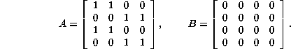
At first sight, the basins for Rules 3 and 252 look completely different, but an examination of these matrices shows why it is sensible to consider them jointly (actually, to pair 252 and 192) - their only difference lies in exchanging the A and the B matrices. Therefore, they will have identical statistics, with 1's and 0's exchanged. In other words, ancestors will proliferate similarly, although their cycles and periods may be different.
The other two operations which the authors consider, reflection and complementation, also have their repercussions. For example, reflection exchanges the start neighborhoods 01 and 10, while complementation does this, exchanges 00 with 11, and exchanges A with B. None of these things changes norms or eigenvalues. Persons familiar with matrix theory will see that the matrices representing these exchanges will commute with the A, B pair, and that they will constitute a symmetry group. A sort of supersymmetry can be achieved by making a bigger matrix having A and B as submatrices, but we will not make further use of the possibility.
There is an extensive theory of positive matrices, just as there is of integer matrices. Matrices in general can be associated with graphs; their nodes are the indices, which are linked according to whether the matrix elements are zero or not. This means that nonzero elements in the product of matrices are associated with chains in the diagram. The relationship is useful when some properties are more evident in one context than in the other. For example, the matrix is partially diagonal when the graph consists of two disjoint parts. Blocks of zeroes correspond to attractors (into which links may enter but cannot leave) and dispersors (links leave but do not enter). Conversely, statistics concerning the graph often have nice matrix formulas, and in general properties of graphs can be worked out in a computer whenever they have a formulation via matrix algebra.
Two important properties of matrices are, on the one hand, their eigenvalues and eigenvectors, and on the other, their norms. The two are related, but the relationship is more complicated when the matrices are not symmetric, so that attractors and dispersors can be present. The norm is not a perfect ``absolute value'' because the norm of a product is only less, not necessarily equal, to the product of norms. For purposes of analysis and calculating limits, the inequality is entirely satisfactory, but it is less favorable when exact counts are required.
The matrices A and B count the ancestors of a single cell, and catalog them according to the start and stop strings constituting the neighborhood. It is a fundamental reality of cellular automata theory that there are always more cells amongst the neighborhoods than the number of cells being considered; this shows itself when we use a matrix rather than a scalar to do our counting. If A and B count the ancestors of a single cell, we expect their products to count the ancestors of a sequence of cells. A matrix is still called for, because marginal cells always remain, however long the chain.
The de Bruijn matrices for (2,1) automata have both norm 2, and largest eigenvalue 2, and these quantities are always larger than those of any of the fragments into which the matrices decompose. The value 2 corresponds to doubling the total number of configurations every time a single cell is added to the automaton.
Consider the formulas for counting (within the limits of pure ASCII). If
M is the connectivity matrix of a graph, let u be a vector of
ones, and i be a unit vector in the ![]() coordinate. Let
coordinate. Let ![]() designate trasnspose. Then i
designate trasnspose. Then i![]() Mj is the
Mj is the ![]() element,
the number of links from i to j, while i
element,
the number of links from i to j, while i![]() Mi is the
number of loops starting at i. Their sum is the Trace of M, yielding
the number of loops altogether (with a possible multiplicity according to
their length). The product u
Mi is the
number of loops starting at i. Their sum is the Trace of M, yielding
the number of loops altogether (with a possible multiplicity according to
their length). The product u![]() Mu is the number of links
altogether, no restriction. q
Mu is the number of links
altogether, no restriction. q![]() Mq is the number of paths
beginning and ending with a quiescent state, q.
Mq is the number of paths
beginning and ending with a quiescent state, q.
All three of these formulae can be written as traces, in the form Tr( GM),
with a suitable metric matrix G. To count everything,
G= uu![]() ; for periodicboundary conditions, G= I, the
unit matrix, and for configurations quiescent at infinity,
G= qq
; for periodicboundary conditions, G= I, the
unit matrix, and for configurations quiescent at infinity,
G= qq![]() . Among other things, this means that the choice of a
boundary condition is not very essential to a calculation. It only enters
at the last moment, in the selection of the metric matrix. But the essential
qualities of the matrix, as represented by its eigenvalues and eigenvectors,
expressing such things as rates of growth, are not affected by the boundary
condition.
. Among other things, this means that the choice of a
boundary condition is not very essential to a calculation. It only enters
at the last moment, in the selection of the metric matrix. But the essential
qualities of the matrix, as represented by its eigenvalues and eigenvectors,
expressing such things as rates of growth, are not affected by the boundary
condition.
Suppose that we want to count configurations. We must add A and B, which
always results in the de Bruijn matrix D (which has a rather simple
characteristic equation - ![]() , because
, because ![]() ,
, ![]() ).
So, for cyclic boundary conditions in a ring of circumference s,
).
So, for cyclic boundary conditions in a ring of circumference s, ![]() ,
which is so unsurprising that it might be considered boring. But it is
almost the only result that we are going to get free.
,
which is so unsurprising that it might be considered boring. But it is
almost the only result that we are going to get free.
Counting is good for getting averages. But suppose we want variances. Then
it is necessary to sum squares. That is where matrix theory is really going
to shine. We need ![]() , which turns out to be
, which turns out to be ![]() ,
which in turn is
,
which in turn is ![]() . Extracting the constant
factor
. Extracting the constant
factor ![]() , we have to calculate
, we have to calculate ![]() . Here
. Here ![]() indicates a tensor product, which is a way of compounding matrices that
will be found in books on matrix theory
indicates a tensor product, which is a way of compounding matrices that
will be found in books on matrix theory![]() .
.
A certain amount algebraic manipulation ends us up with a formula for the
second moment when the de Bruijn matrix is split into A and B; namely we
need a trace involving ![]() , (rather than
, (rather than ![]() )
in a ring of circumference s. These commentaries aren't the place for
mathematical derivations, but the details are available in a pair of
preprints
)
in a ring of circumference s. These commentaries aren't the place for
mathematical derivations, but the details are available in a pair of
preprints![]() that anyone can have by sending a mailing address
(including zip code, city, country, etc).
that anyone can have by sending a mailing address
(including zip code, city, country, etc).
A tensor square has an interpretation as a graph; it is nothing other than the graph of ordered pairs taken from the graph of the original matrix. (There is also a symmetrized tensor square, and an unordered-pair graph). This relationship is intimately related to Niall Graham ( niall@nmsu.edu)'s assertion of 21 Jun 93 14:55:27:
>
> A 1-dim CA is reversible iff the pair digraph of its
> associated finite automaton is acyclic.
>
More commentary will follow.