The Weyl-Titchmarsh m-function

Once that it has been established that there are resonances, it becomes a question of how to treat them analytically. Strictly speaking, this should be done for complex energies even though the differential equation is real, because there is a criterion for boundedness and unboundedness and a way of working with square-integrable solutions.

In practice, most of the information can be gotten from an examination of the real solutions, the only substantive question being the one of evaluating the amplitude at infinity for continuum wave functions. Symmetry can be a considerable asset, when it is present, because the solutions will fall into irreducible representations of the symmetry group. Thus for a harmonic oscillator well centered at the origin, solutions can be either even or odd.

If the prolongation of a symmetric solution has components $A\cos\theta, B \sin\theta$ , the traditional substitution

R	=	$\displaystyle \sqrt(A^2+B^2)$	(13)
$\displaystyle \delta$	=	$\displaystyle \arctan(B/A)$	(14)

More complete details of this procedure can be found in the differential equation textbook of Coddington and Levinson [9], which is one of the very few which take up the topic of spectral densities and spectral matrices. Generalities, including a fair part of the treatment of the Dirac harmonic oscillator which is repeated here, can be found in McIntosh's contribution to Loebl's second volume on group theory [7]. The explicit reduction of the boundary value problem into three levels of symmetry, including the spectral distribution matrix, can be found in his contribution to Löwdin's Festschrift [8].

Figure 5 shows a hidden surface plot of the reciprocal of R around one of the resonances of the Dirac harmonic oscillator. Actually, having used R to normalize the wave function, the quantity which is graphed is the probability amplitude, which, for the Dirac equation, is the sum of the squares of the two components of the wave function.

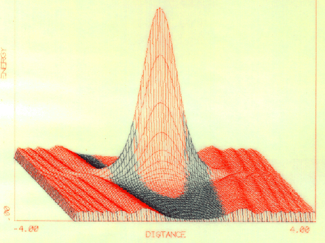**Figure 5:** The region colored in black is the clasically forbidden region, where the wave function is exponential.
$\begin{figure} \centering \begin{picture} (406,320) \put(0,0){\epsfxsize=406pt \epsffile{dirac.eps}} \end{picture} \end{figure}$

This graph is one of many produced by the PDP-10 program <PLOT75>, this one exploiting the use of colored pens to color the resonance peak according to the location of the clasically forbidden region. This is the region in which the phase of the wave function at the classical turning point decides whether it will grow or shrink as it crosses the forbidden region, and emerging at the other classical turning point, fixes the amplitude of the wave function in the antiparticle region.

Since surface coloring can be used to exhibit whatsoever property of the wave function, Figure 6 is used to show the phase of the wave function rather than the square of its amplitude.

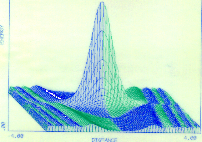**Figure 6:** Although the surface represents probabilities, it is colored according to the phase of the wave function.
$\begin{figure} \centering \begin{picture} (406,320) \put(0,0){\epsfxsize=406pt \epsffile{new-2.eps}} \end{picture} \end{figure}$

The object displayed in the figure is the resonance peak corresponding to what would be the ground state in the nonrelativistic or infinite-mass limit. It therefore resembles a cosine (more precisely, a gaussian) and is even. The quantity coloring the surface is evidently the situation of the solution vector in the left or right half of the phase plane so that each undulation of the surface carrise the point halfway around the origin.

The most instructive feature of all these graphs is the phase change of the wave function with increasing energy on passing a resonance peak. Crests in the wave surface follow the parabolic potential at a respectful distance, but a a new crest is born at each resonance and pushes the others out, further away from the forbidden region. In other words, an $180^\circ$ phase shift accompanies each resonance crossing.

Another detail to be noticed is the rapidity with which the undulations die down to a fairly constant height, which of course is their asymptotic value. But they wiggle faster and faster, this being due to the x³ factor dominating their phase.

In Figure 7 the same surface is repeated once again, this time colored in bands of constant energy increment. There is no reason why a checkerboard could not have been built up, by switching colors following a constant increment in x, but such things have to be planned before making the graph, not afterwards.

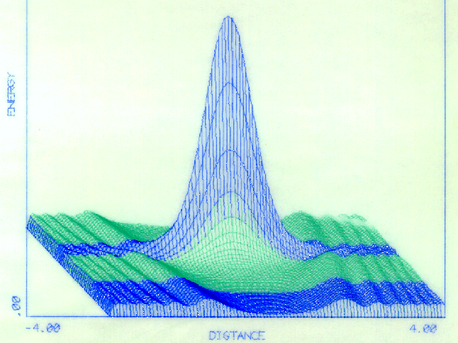**Figure 7:** Although the surface represents probabilities, it is colored according the value of the energy, in strips of unit increment, thereby allowing a quick estimate of the eigenvalues.
$\begin{figure} \centering \begin{picture} (406,320) \put(0,0){\epsfxsize=406pt \epsffile{new-1.eps}} \end{picture} \end{figure}$

Since one band nicely straddles the peak, the flow of crests in the antiparticle region still receives its nudge from the resonance, with its impact on the artistic value of the picture.

Although they are not always planned, artifacts of the drawing program frequently induce elements of texture into the image they are producing. Sometimes the result is only a pleasing apearance, something which turns out to be rather subjective. Other times, the moirés produced reveal the flatness of the image, or abrupt changes such as edges, depressions, or protrusions. If the moiré is very regular, that is evidence that the image is quite smooth.

Useful as perspective drawings with hidden line suppression are for visualizing phenomona, they are still complementary to contour maps, such as the one shown in Figure 8, which encompasses three successive resonances, starting with the one depicted in the previous Figures. It was an ezperiment, using a thick pointed pen with colored ink to try to fill in an area rather than simply mark out lines.

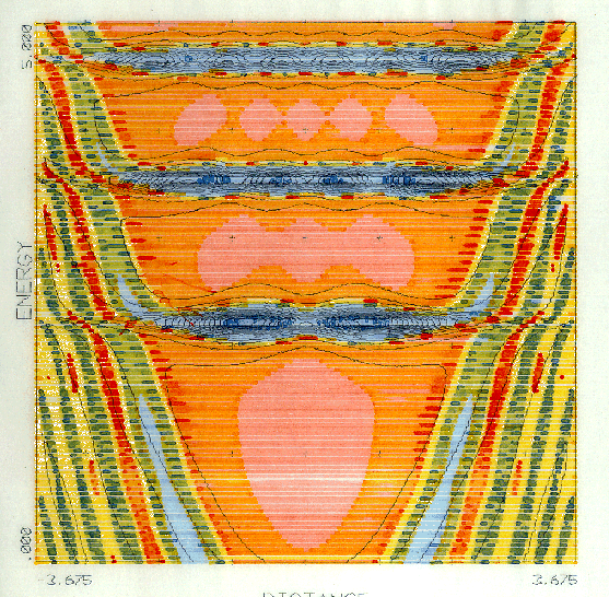**Figure 8:** Contour map of the probability density for the odd solutions of the Dirac harmonic oscillator equation. There would be a corresponding map for the odd solution. Since the potential is symmetric, we know that parity determines the eigenfunctions,without having to diagonalize the spectral density matrix.
$\begin{figure} \centering \begin{picture} (350,360) \put(0,10){\epsfxsize=350pt \epsffile{new-3.eps}} \end{picture} \end{figure}$

Because of the parity of the initial condition, contour maps such as these show either the even resonances or the odd resonances. The vertical viewpoint shows the flow of crests around resonances quite clearly. Notice that the antiresonances have just as much interior structure as the resonances; in fact there is a fairly reciprocal relationship for amplitudes.

In some versions of this drawing, the classically forbidden region has been overlaid, showing quite clearly that all the crest shifting goes one in and at the margins of that region.

Returning to perspective drawings, Figure 9 encompasses a broader range of peaks, more in keeping with the range of the contour map.

**Figure 9:** Probability amplitudes for even (lower image) and odd (upper image) solutions.
$\begin{figure} \centering \begin{picture} (400,390) \put(0,0){\epsfxsize=400pt \... ...}} \put(0,205){\epsfxsize=400pt \epsffile{new-5.eps}} \end{picture} \end{figure}$

Much planning can, or at least should, go into preparing drawings of functions. For example, the angle of view and relative compactness of Figure 9 allows further insight into the crest arrangement of the Dirac harmonic oscillator. Some conclusions can be drawn about the relative amplitudes of the different resonances, but it should not be supposed that they are normalized. On the contrary, their defining characteristic is unit amplitude at infinity. Under those circumstances none of the solutions can be normalized, and the most that can be expected is that they will play their part in the definition of the spectral density function via the Stieltjes integral.